Getting Started¶

odelab is a Python library for solving differential equations.

There is support for

easily solving generic differential equations using one of the many methods already provided in odelab
solve differential equations of a special structure, such as differential-algebraic equations, and equations arising in mechanics
easily create your own custom numerical schemes

Differential Equations¶

Differential Equations in Mathematics¶

A differential equation is a problem of the following kind. One is looking for a function \(u\) which fulfills the following property:

\[u'(t) = f(t,u(t)) \qquad \forall t ≥ 0\]

Such a problem has many solutions, so one must also prescribe an initial condition:

\[u(0) = u_0\]

The data of the function \(f\) and of the initial condition \(u_0\) guarantee in general the existence and uniqueness of the solution.

Solving Differential Equations Numerically¶

In order to solve a differential equation numerically, we need a numerical scheme. The simplest numerical scheme is the explicit Euler method, described as follows:

\[u_{n+1} = u_{n} + h f(t_n, u_n)\]

Given an initial condition \(u_0\), the explicit Euler method successively creates \(u_1\), \(u_2\), etc. Notice that one has to specify a time step \(h\) for this method to work.

odelab comes with many such schemes, and makes it very easy to create new ones, see Scheme.

Step-by-step Example¶

Let us examine a simple example. Suppose we want to solve the problem

\[u' = -u\]

with the initial condition

\[u(0) = u_0 = 1\]

We first have to define the system, that is, the right hand side of the differential equation. This is done as follows:

from odelab import System

def f(t,u):
    return -u

system = System(f)

The next thing we need is to choose a numerical method to solve that differential equation. Let us choose a very simple scheme, the explicit Euler scheme. Most numerical schemes require a time step. We choose here a time step of \(0.1\). This is done as follows:

from odelab.scheme.classic import ExplicitEuler
scheme = ExplicitEuler(0.1) # Explicit Euler scheme with time step 0.1

Now we have to set-up a solver object that will take care of running the simulation and storing the resulting computations:

from odelab import Solver
s = Solver(scheme=scheme, system=system) # we use the scheme and system variables defined earlier

We still need to specify the initial condition for this simulation:

s.initialize(u0=1.)

Finally, we can run the simulation from \(t=0\) to \(t=1\) with the following call:

s.run(1.)

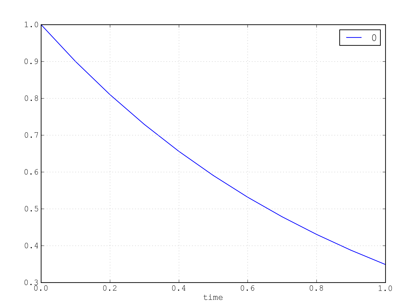
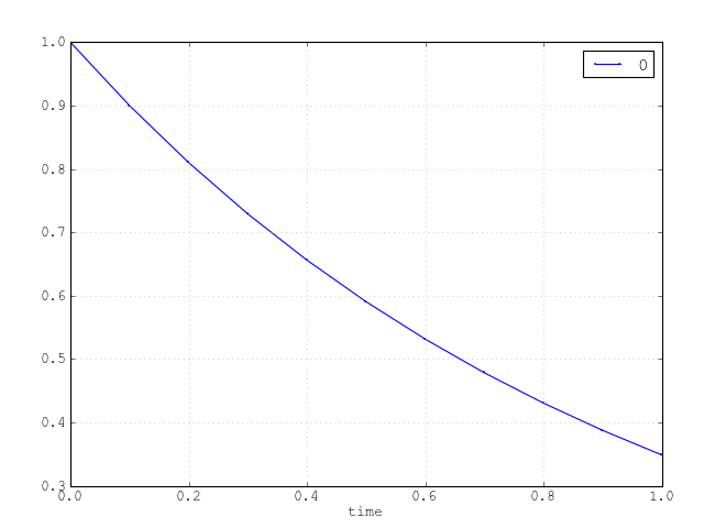
To summarize what we have up to now, the whole code is the following:

from odelab import Solver, System
from odelab.scheme.classic import ExplicitEuler

def f(t,u):
    return -u

s = Solver(scheme=ExplicitEuler(.1), system=System(f))
s.initialize(u0=1.)
s.run(1.)

s.plot()

[source code, hires.png, pdf]

Example with Plot¶

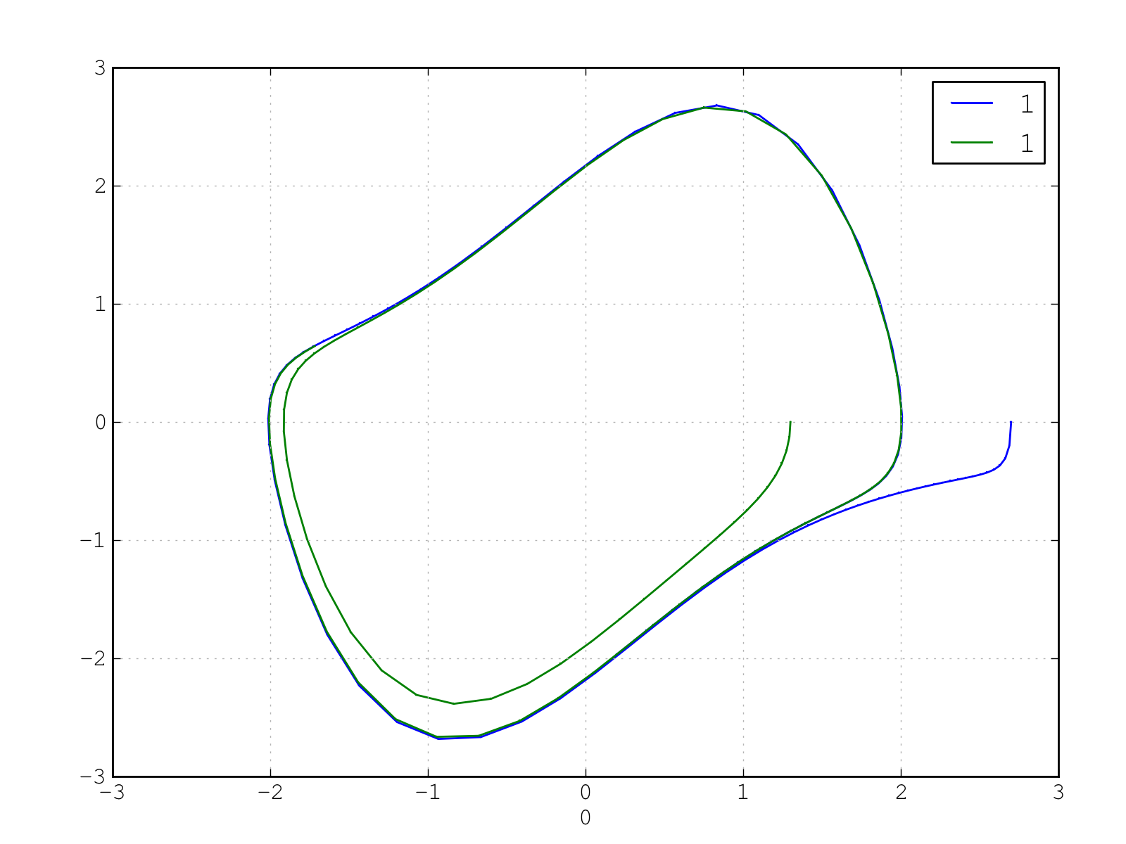
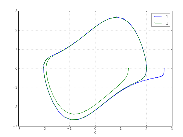
Example: Solving the van der Pol equation

Here is an example of solving the van der Pol equations with a Runge-Kutta method and then plotting the result with plot2D. See Simulation Name and 2D Plot for more information.

from odelab import Solver
from odelab.scheme.classic import RungeKutta4
from odelab.system.classic import VanderPol

s = Solver(scheme=RungeKutta4(.1), system=VanderPol())
s.initialize([2.7,0], name='2.7')
s.run(10.)
s.plot2D()

s.initialize([1.3,0], name='1.3')
s.run(10.)
s.plot2D()

[source code, hires.png, pdf]

Architecture¶

odelab is built on a very simple architecture. The main classes are Solver, Scheme and System.

Solver takes care of initializing, running and storing the result of a simulation

System models a right hand side, which may be just a function, or a partitioned system, or even a DAE.

Scheme models a method to solve the equation. It may be explicit or implicit, adaptive or not, it is all up to you.